Regression

Linear Regression

In machine learning, we often want to predict continuous numerical values, like house prices, temperatures or sales figures. Linear regression also knows as Ordinary Least Squares (OLS) provides a foundational approach to this problem by modeling the relationship between input variables and a target variable using a straight line.

This chapter introduces linear regression through a hands-on example. You'll learn to:

• Build and train a linear regression model
• Interpret model parameters (intercept and coefficients)
• Make predictions with new data
• Evaluate model performance using the coefficient of determination (\(R^2\))
• Get familiar with the scikit-learn workflow to train and evaluate models

---

Info

This chapter adapts and expands upon:

• scikit-learn: Ordinary Least Squares and Ridge Regression
• scikit-learn: Linear Models
• scikit-learn: Metrics and scoring: quantifying the quality of predictions

Theory

Linear regression, also known as Ordinary Least Squares (OLS), models the relationship between a continuous target variable \(y\) and one or more input variables \(X\). The goal is to find the best linear function that predicts \(\hat{y}\) from \(X\).

Linear combination

\[ \hat{y} = w_0 + w_1 \cdot x_1 + w_2 \cdot x_2 + ... + w_n \cdot x_n \]

where:

• \(w_0\) is the intercept (bias term)
• \(w_1, w_2, ..., w_n\) are the coefficients (weights)
• \(x_1, x_2, ..., x_n\) are the input features

The term "Ordinary Least Squares" refers to the optimization objective, finding the weights \(w_0, w_1, ..., w_n\) that minimize the sum of squared differences called residuals between the actual values \(y\) and predicted values \(\hat{y}\).

Cost function

\[ \text{min} \quad \sum_{i=1}^{n} (y_i - \hat{y}_i)^2 \]

where \(n\) is the number of observations.

This minimization ensures that our model makes the smallest possible errors on average when predicting the training data. Let's look at an example.

Example

scikit-learn provides a couple of data sets for download. To fit a linear regression on a real-world example, we choose the California housing data set. More information about the California Housing data set can be found here.

Info

Data reference:

Pace, R. Kelley and Ronald Barry, Sparse Spatial Autoregressions, Statistics and Probability Letters, 33:291-297, 1997

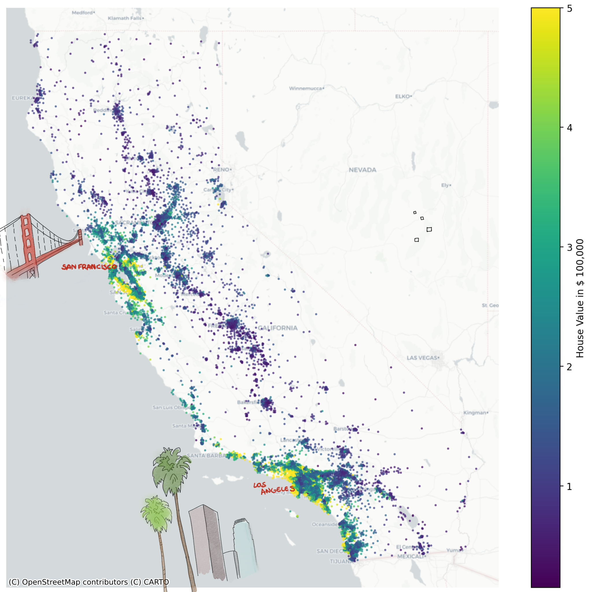
Our objective is to model the target variable \(y\) using input variables \(X\). In this case, \(y\) corresponds to the median house value, expressed in hundreds of thousands of dollars ($100,000). Below figure shows all houses in California colored by their median value \(y\).

California median house values (in $100,000): Higher values are concentrated along the coast and in major urban centers such as San Francisco and Los Angeles.

Load the data

Start by loading the data:

from sklearn.datasets import fetch_california_housing

X, y = fetch_california_housing(return_X_y=True, as_frame=True)
print(X.head())

Conveniently, by setting return_X_y=True, the function splits the input variables \(X\) and the target \(y\). Note, \(X\) contains multiple input variables such as such as house age HouseAge and average bedrooms AveBedrms. However, some are not needed.

Question

The data frame X contains the variables "Latitude" and "Longitude", remove them from the data frame. Tip: Consult the pandas documentation.

Split the data

Before training our OLS model, we need to split our data into two distinct sets:

• Training set: Used to fit the model and learn the optimal weights (80% of data)
• Test set: Used to evaluate the model's performance on unseen data (20% of data)

Think of this like preparing for an exam: you study from practice problems (training set) and then test your knowledge with new questions (test set). This separation allows us to assess whether our model can accurately predict house prices it hasn't seen before, rather than just memorizing the training data.

Info

The 80/20 split is a common convention, but not a strict rule. Depending on the data set size, other split ratios might be a better fit.

from sklearn.model_selection import train_test_split

X_train, X_test, y_train, y_test = train_test_split(
    X, y, test_size=0.2, random_state=42, shuffle=True
)

Let's break the code snippet down:

1. train_test_split() takes the complete data set (X and y) as input
2. Splits off 20% for testing (test_size=0.2)
3. Randomly shuffles the data (shuffle=True) to remove any inherent ordering
4. Set a seed (random_state=42) which ensures the same outcome every time the code snippet is executed. Since the shuffle operation is stochastic, we aim for reproducibility.

Why shuffle?

Some data sets may have inherent order (e.g., the houses could be sorted by location). Shuffling ensures that both training and test sets are representative of the entire data distribution.

After splitting, we put our test data (X_test and y_test) aside and use it at the very end to measure the model's performance.

Intuition

For the first OLS model, we use a single input variable \(X\) as it allows us to easily visualize and interpret the results. The choice falls on the median income at the house location, referred to as MedInc. Visualize the target and input variable in a scatter plot:

import matplotlib.pyplot as plt

fig, ax = plt.subplots()
ax.scatter(X_train["MedInc"], y_train, color="#009485")
ax.set(
    xlabel="Input Variable (MedInc)",
    ylabel="Target (House Value)",
    title="Train set",
)
plt.show()

• Scatter Plot

  ---

  Looking at the scatter plot, you might intuitively imagine drawing a straight line through the points that best captures the trend. This intuition is exactly what OLS does mathematically, it finds the optimal line that minimizes the distance between the line and all data points.

• 

• 

• Best-Fit Line

  ---

  The OLS model finds the line that minimizes the sum of squared residuals, the vertical distances between each point and the line. Recall from the theory section that this is exactly what the cost function measures:

  \[ \text{min} \quad \sum_{i=1}^{n} (y_i - \hat{y}_i)^2 \]

Train the model

Our next step is to train an OLS model to automatically find this "best-fit" line. Remember, since we have one input variable, the linear combination simplifies to:

\[ \hat{y} = w_0 + w_1 \cdot x_1 \]

where:

• \(\hat{y}\) is the predicted house price
• \(w_0\) is the intercept (baseline house price)
• \(w_1\) is the coefficient for the input variable MedInc (\(x_1\))

Start by importing the linear regression model from the package.

from sklearn.linear_model import LinearRegression

# create an instance
model = LinearRegression()

At this point, the model is not trained, however that can be easily done using the fit() method. Remember, to use the training set

model.fit(X=X_train[["MedInc"]], y=y_train)

Intercept and coefficient

After training, we can inspect the model's learned parameters. The intercept and coefficient that define the best-fit line:

print(f"Intercept (w₀): {round(model.intercept_, 4)}")
print(f"Coefficient (w₁): {round(model.coef_[0], 4)}")

>>> Output

Intercept (w₀): 0.4446
Coefficient (w₁): 0.4193

These values tell us that our linear model is:

\[ \hat{y} = 0.4446 + 0.4193 \cdot x_1 \]

Interpretation:

• Intercept (0.4446): The baseline house value (when MedInc is zero) is around $44,460
• Coefficient (0.4193): For each unit increase in MedInc, the house value increases by ~ $41,930

Predictions

Now that the model is trained, we can predict house prices for new observations. Let's predict the price \(\hat{y}\) for a house in an area where MedInc is 3.5:

import pandas as pd

new_house = pd.DataFrame({"MedInc": [3.5]})
# predict returns a numpy array
new_price = model.predict(new_house)
# access first and only element
print(round(new_price[0], 4))

>>> Output

1.9123

The model predicts a house value of approximately $191,230.

Manual validation

We can verify this prediction using our linear equation. Substituting \(x_1 = 3.5\):

\[ \begin{align} \hat{y} &= 0.4446 + 0.4193 \cdot 3.5 \\ &= 1.9122 \end{align} \]

This matches our model's prediction!

Practice: Make your own prediction

Calculate the predicted house price for an area where MedInc is 5.0.

1. Use model.predict() to get the prediction.
2. Validate it by hand using the linear equation.
3. Do the results match?

Evaluate the model

Now we can make predictions, but we don't know how accurate they actually are. We need to quantify the model's performance to determine if it generalizes well to new, unseen data.

Remember we set aside our test set earlier? This is where we use it. By evaluating on data the model hasn't seen during training, we get an honest assessment of its predictive power.

To measure the model's performance, we'll use the coefficient of determination.

Coefficient of determination

Info

This section focuses on the definition implemented by scikit-learn.

The coefficient of determination, known as the \(R^2\) score, measures the proportion of variance in the target variable that is explained by the model.

\(R^2\) Score

\[ R^2(y, \hat{y}) = 1 - \frac{\sum_{i=1}^{n} (y_i - \hat{y}_i)^2}{\sum_{i=1}^{n} (y_i - \bar{y})^2} \]

where:

• \(y_i\) are the actual values
• \(\hat{y}_i\) are the predicted values
• \(\bar{y}\) is the mean of actual values

Interpretation:

• \(R^2 = 1\): Perfect predictions (model explains all variance)
• \(R^2 = 0\): Model performs no better than simply predicting the mean
• \(R^2 < 0\): Model performs worse than predicting the mean

Let's calculate the \(R^2\) score for our model on the test set:

from sklearn.metrics import r2_score

# make predictions on test set
y_pred = model.predict(X_test[["MedInc"]])

# calculate R² score
r2 = r2_score(y_true=y_test, y_pred=y_pred)
print(f"R² Score: {round(r2, 4)}")

>>> Output

R² Score: 0.4589

Understanding \(R^2\)

An \(R^2\) score of 0.4589 means the model explains 45.89% of the variance in house prices using only median income. While this is informative, it's not great. It suggests that other factors (location, house size, etc.) significantly influence house prices.

Find a better model

Can you improve the \(R^2\) score? Fit new models and experiment with the following:

Model variations:

• Use different individual input variables (e.g., HouseAge, AveRooms, AveBedrms)
• Use a combination of multiple input variables
• Compare single-variable vs. multi-variable models

Data preparation:

• Adjust the train-test split ratio
• Remember to use random_state for reproducibility

Analysis:

• Calculate and compare \(R^2\) scores for each model
• Inspect the intercept and coefficients for multi-variable models
• Make predictions with your best-performing model
• Manually verify one prediction using the linear equation

Which combination gives you the highest \(R^2\) score? What does this tell you about which features are most important for predicting house prices?

Detour: Model workflow

The workflow you practiced here forms the foundation for all supervised learning algorithms in scikit-learn:

# 1. Split your data
X_train, X_test, y_train, y_test = train_test_split(X, y, ...)

# 2. Import and instantiate a model
model = SomeModel()

# 3. Train the model
model.fit(X_train, y_train)

# 4. Make predictions
y_pred = model.predict(X_test)

# 5. Evaluate performance
score = model.score(y_test, y_pred)

This consistent pattern applies to all upcoming chapters, whether you're building regression or classification models.

Recap

In this chapter, you learned the fundamentals of linear regression through a practical example. The key takeaways:

• Linear regression models the relationship between input variables and a target variable using a linear combination. Find the best-fit line by minimizing the sum of squared residuals.
• \(R^2\) score quantifies how well the model explains variance in the target variable
• scikit-learn workflow allows to easily train and evaluate model